Fangraphs recently published an interesting dataset that measures defensive efficiency of fielders. For each player, the Inside Edge dataset breaks their opportunities to make plays into five categories, ranging from almost impossible to routine. It also records the proportion of times that the player successfully made the play. With this data, we can see how successful each player is for each type of play. I wanted to think of a way to combine these five proportions into one fielding metric. From here on, I will assume that there is no error in categorizing a play as easy or hard and that there is no bias in the categorizations.
Model
The model I will build is motivated by ordinal regression. If we only were concerned with the success rate in one of the categories, we could use standard logistic regression, and the probability that player $i$ successfully made a play would be assumed to be $\sigma(\theta_i)$, where $\sigma()$ is the logistic function. Using our prior knowledge that plays categorized as easy should have a higher success rate than plays categorized as difficult, I would like to generalize this.
Say there are only two categories: easy and hard. We could model the probability that player $i$ successfully made an hard play as $\sigma(\theta_i)$ and the probability that he made an easy play as $\sigma(\theta_i+\gamma)$. Here, we would assume that $\gamma$ is the same for all players. This assumption implies that if player $i$ is better than player $j$ at easy plays, he will also be better at hard plays. This is a reasonable assumption, but maybe not true in all cases.
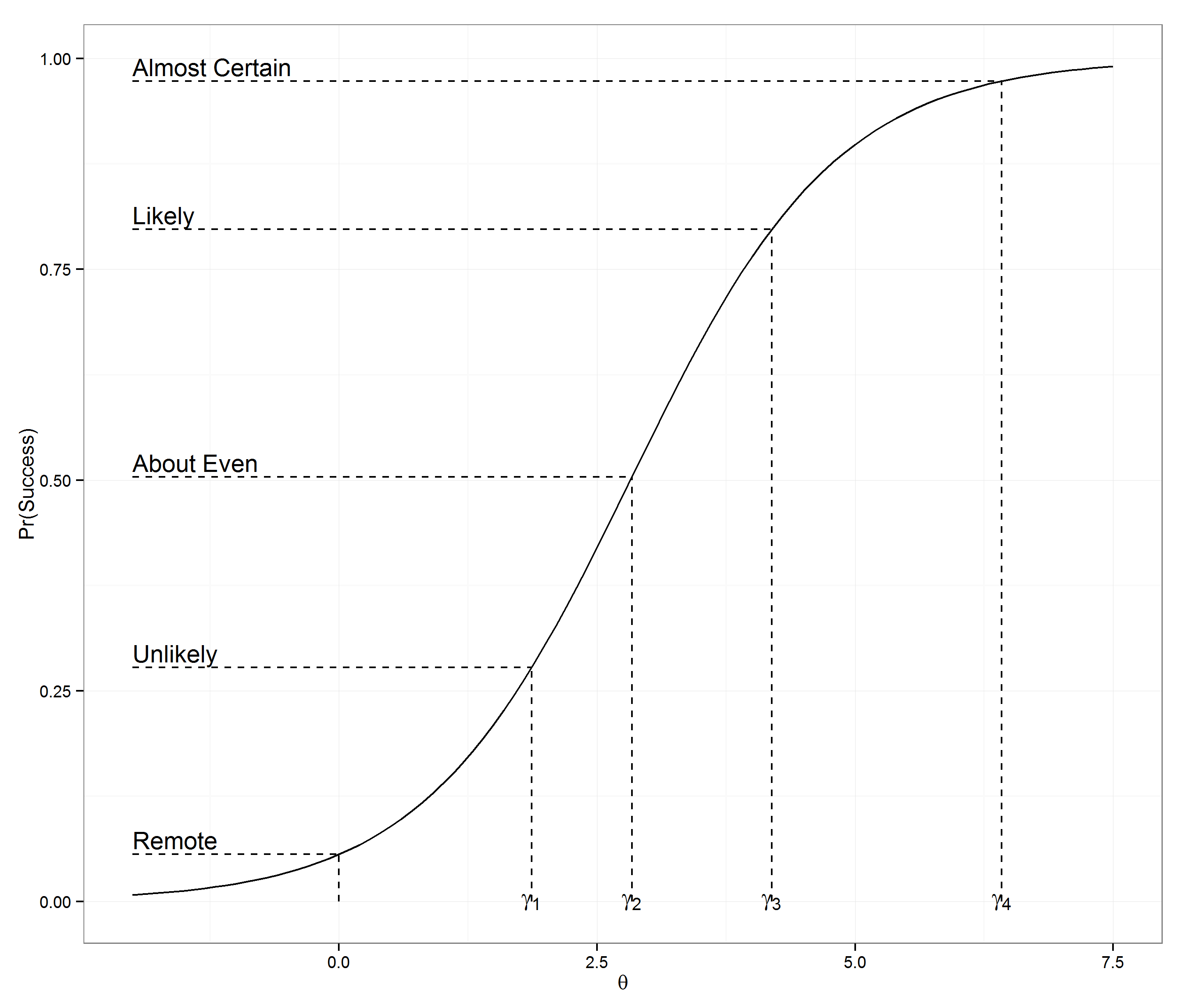
Since we have five different categories of difficulty, we can generalize this by having $\gamma_k, k=1,\ldots,4$. Again, these $\gamma_k$’s would be the same for everyone. A picture of what this looks like for shortstops is below. In this model, every player will effectively be shifting the curve either left or right. A positive $\theta_i$ means the player is better than average and cause the curve to shift left and vice versa for negative $\theta_i$.
I modeled this as a multi-level mixed effects model, with the players being random effects and the $\gamma_k$’s being fixed. Technically, I should optimize subject to the condition that the $\gamma_k$’s are increasing, but the unconstrained optimization always yields increasing $\gamma_k$’s because there is a big difference between success rate in the categories. I used combined data from 2012 and 2013 seasons and included all players with at least one success and one failure. I modeled each position separately. Modeling player effects as random, there is a fair amount of regression to the mean built in. In this sense, I am more trying to estimate the true ability of the player, rather than measuring what he did during the two years. This is an important distinction, which may differ from other defensive statistics.
Model fit
Below is a summary of the results of the model for shortstops. I am only plotting the players with the at least 800 innings, for readability. A bonus of modeling the data like this is that we get standard error estimates as a result. I plotted the estimated effect of each player along with +/- 2 standard errors. We can be fairly certain that the effects for the top few shortstops is greater than 0 since their confidence intervals do not include 0. The same is true for the bottom few. Images for the other positions can be found here.
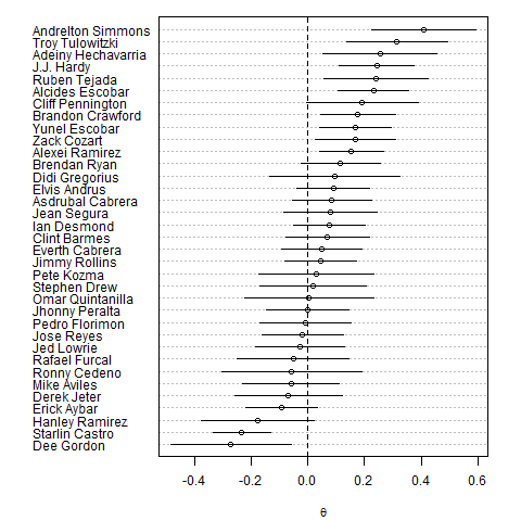
The results seem to make sense for the most part. Simmons and Tulowitzki have reputations as being strong defenders and Derek Jeter has a reputation as a poor defender.
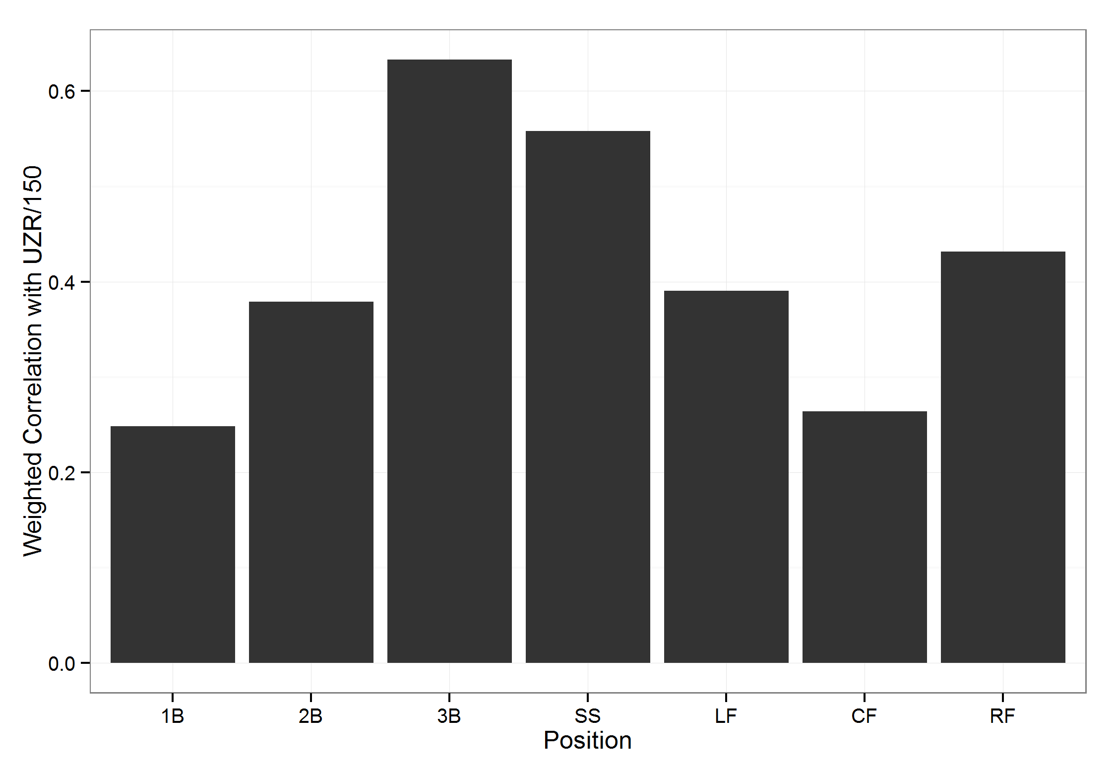
Further, I can validate this data by comparing it to other defensive metrics. One that is readily available on Fangraphs is UZR per 150 games. For each position, I took the correlation of my estimated effect with UZR per 150 games, weighted by the number of innings played. Pitchers and catchers do not have UZR’s so I cannot compare them. The correlations, which are in the plot below, range from about 0.2 to 0.65.
Interpreting parameters
In order to make this fielding metric more useful, I would like to convert the parameters to something more interpretable. One option which makes a lot of sense is “plays made above/below average”. Given an estimated $\theta_i$ for a player, we can calculate the probability that he would make a play in each of the five categories. We can then compare those probabilities to the probability an average player would make a play in each of the categories, which would be fit with $\theta=0$. Finally, we can weight these differences in probabilities by the relative rate that plays of various difficulties occur.
For example, assuming there are only two categories again, suppose a player has a 0.10 and 0.05 higher probability than average of making hard and easy plays, respectively. Further assume that 75% of all plays are hard and 25% are easy. On a random play, the improvement in probability over an average player of making a play is $.10(.75)+.05(.25)=0.0875$. If a player has an opportunity for 300 plays in an average season, this player would be $300 \times 0.0875=26.25$ plays better than average over a typical season.
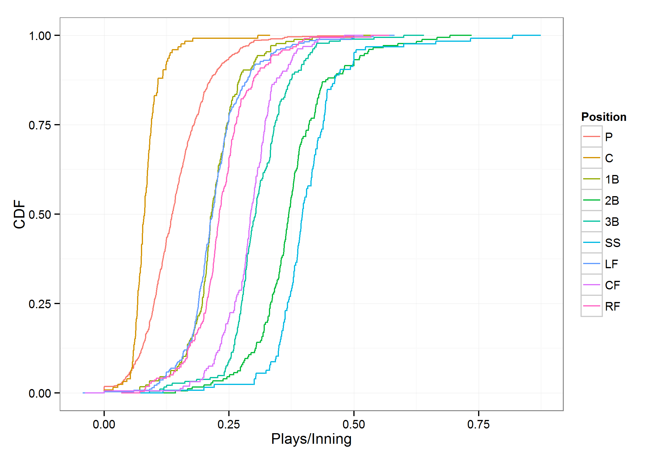
I will assume that the number of opportunities to make plays is directly related to the number of innings played. To convert innings to opportunities, I took the median number of opportunities per inning for each position. For example, shortstops had the highest opportunities per inning at 0.40 and catchers had the lowest at 0.08. The plot below shows the distribution of opportunities per inning for each position.
We can extend this to the impact on saving runs from being scored as well by assuming each successful play saves $x$ runs. I will not do this for this analysis.
Results
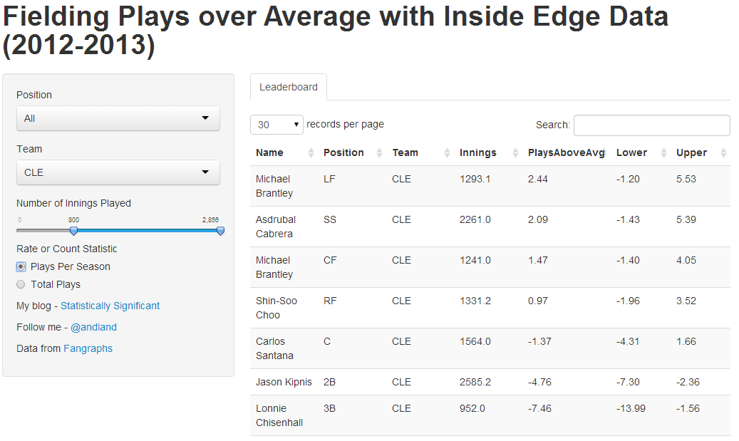
[Update: The Shiny app is no longer live, but you can view the resulting estimates in the Github repository.]
Finally, I put together a Shiny app to display the results. You can search by team, position, and innings played. A team of ‘- - -’ means the player played for multiple teams over this period. You can also choose to display the results as a rate statistic (extra plays made per season) or a count statistic (extra plays made over the two seasons). To get a seasonal number, I assume position players played 150 games with 8.5 innings in each game. For pitchers, I assumed that they pitched 30 games, 6 innings each.
Conclusions and future work
I don’t know if I will do anything more with this data, but if I could do it again, I may have modeled each year separately instead of combining the two years together. With that, it would have been interesting to model the effect of age by observing how a player’s ability to make a play changes from one year to the next. I also think it would be interesting to see how changing positions affects a players efficiency. For example, we could have a $9 \times 9$ matrix of fixed effects that represent the improvement or degradation in ability as a player switches from their main position to another one. Further assumptions would be needed to make sure the $\theta$’s are on the same scale for every position.
At the very least, this model and its results can be considered another data point in the analysis of a player’s fielding ability. One thing we need to be concerned about is the classification of each play into the difficultness categories. The human eye can be fooled into thinking a routine play is hard just because a fielder dove to make the play, when a superior fielder could have made it look easier.
Code
I have put the R code together to do this analysis in a gist. If there is interest, I will put together a repo with all the data as well.
Update: I have a Github repository with the data, R code for the analysis, the results, and code for the Shiny app. Let me know what you think.