CD1025’s Playlist and Summerfest

Last time, I showed you how to download CD1025’s playlist back to last year and did some exploratory analysis to find that there were some gaps in the data. Using this data, I would like to look at the artists that are playing in this week’s Summerfest. Summerfest is one of the biggest shows that CD1025 puts on every year and is hyped quite a bit on the station. I would like to look into whether they play the headliners more once they have booked the artists.

I am going to concentrate on data from January 1st and on so I don’t include too much irrelevant data. Below is a function where I can input a number related to which headliner I want and it will plot the plays per day of that artist from January 1st to the most recent history. I also plot a smooth curve and a vertical line when the lineup was announced on June 24th.

playlist=subset(playlist,Day>=mdy("1/1/13"))
plays.per.day=sqldf("Select Day, Count(Artist) as Num
      From playlist
      Group By Day
      Order by Day")
summerfest.artists=c("MATT AND KIM","COLD WAR KIDS","RA RA RIOT","SMITH WESTERNS",
                       "J. RODDY WALSTON AND THE BUSINESS","CAYUCAS",
                       "THAO AND THE GET DOWN STAY DOWN","DALE EARNHARDT JR. JR.")

plot.plays <- function(artist.num) {
  summerfest=summerfest.artists[artist.num]
  song.per.day=sqldf(paste0("Select Day, Count(Artist) as Num
                      From playlist
                      Where Artist='",summerfest,"'
                      Group By Day
                      Order by Day"))
  song.per.day=merge(plays.per.day[,1,drop=FALSE],song.per.day,all.x=TRUE)
  song.per.day$Num[is.na(song.per.day$Num)]=0
  
  qplot(Day,Num,data=song.per.day,geom="point")+labs(x="Date",y="Plays",title=summerfest,colour=NULL)+
    geom_vline(xintercept=as.numeric(mdy("6/24/13")),lty=2)+
    geom_smooth(method="gam",family=poisson,formula=y~s(x),se=F,aes(colour="Smooth"),size=2)
}

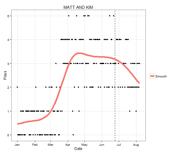
Doing this with the first artist, Matt and Kim, you can see that the plays per day steadily increased sharply some time in late March and stayed about constant there until the announcement. After the announcement, surprisingly, the plays have decreased. The fact that the plays increased in late March indicates to me that it is possible that they booked Matt and Kim then and increased them in the rotation in order to make the band more familiar to the audience. Of course, there are many other (possibly more reasonable) reasons that the play count increased, so I may be reading into it too much.

plot.plays(1)

I would like to statistically determine when the number of plays changed the most and from that infer when the station had booked the artist. To do this I assume a change point model. Since we are dealing with counts, I will assume that the number of plays in a day follows a Poisson distribution. In a change point model, there is some day, $\tau$, where the mean parameter of the Poisson distribution changes. Before that date, the play counts follow a Poisson with mean $\lambda_1$ and after the mean is $\lambda_2$ ($\lambda_1 \neq \lambda_2$).

Let $X_i$ be the number of plays for Matt and Kim on date $i$. The generative model is

$$ X_i \sim Poisson(\lambda_1), i \leq \tau$$

$$X_i \sim Poisson(\lambda_2), i > \tau$$

and therefore the likelihood is

$$\prod_{i=\text{Jan 1}}^{\tau-1} \frac{\lambda_1^{x_i}}{x_i !} e^{\lambda_1}$$

$$\prod_{i=\tau}^{\text{June 23}} \frac{\lambda_2^{x_i}}{x_i !} e^{\lambda_2}$$

If $\tau=t$ is known, maximizing the likelihood with respect to $\lambda_1$ and $\lambda_2$ is easy.

$$\hat{\lambda}_1 = \bar{x}[\leq t]$$

$$\hat{\lambda}_2 = \bar{x}[> t]$$

which are the average play counts per day before and after $t$.

We can easily find the $\hat{\tau}$ that maximizes the likelihood by looping $t$ through every day from January 1 to June 22, finding the maximum likelihood estimates, and calculating the likelihood. The $t$ that gives the highest likelihood and the corresponding $\lambda$s are the MLEs. A function for the maximized log likelihood is given below for a given $t$.

log.like.known = function(t) {
    pre = song.per.day$Day <= t
    post = song.per.day$Day > t & song.per.day$Day < mdy("6/24/13")
    lambda1hat = sum(song.per.day$Num[pre])/sum(pre)
    lambda2hat = sum(song.per.day$Num[post])/sum(post)
    sum(song.per.day$Num[pre]) * log(lambda1hat) + sum(song.per.day$Num[post]) * 
        log(lambda2hat) + -sum(pre) * lambda1hat - lambda2hat * sum(post)
}

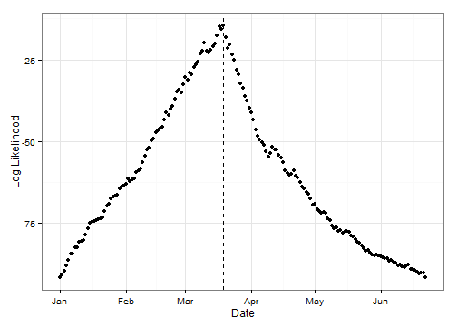
In the code below, I plot the maximized log likelihood for every given $\tau$. You can see that it peaks in the middle of March (March 19th to be specific).

summerfest=summerfest.artists[1]
song.per.day=sqldf(paste0("Select Day, Count(Artist) as Num
                    From playlist
                    Where Artist='",summerfest,"'
                    Group By Day
                    Order by Day"))
song.per.day=merge(plays.per.day[,1,drop=FALSE],song.per.day,all.x=TRUE)
song.per.day$Num[is.na(song.per.day$Num)]=0

dts=seq(mdy(01012013),mdy(06222013),by="1 day")
loglikes=sapply(dts,log.like.known)
tauhat=dts[which.max(loglikes)]
qplot(dts,loglikes)+geom_vline(xintercept=as.numeric(tauhat),lty=2)+
  labs(x="Date",y="Log Likelihood")

Combining this information with the previous plot, we can visualize our break point model. First I recalculate the $\lambda$s now that the $\hat{\tau}$ is known. Then I plot the fitted model on the previous plot.

pre=song.per.day$Day<=tauhat
post=song.per.day$Day>tauhat & song.per.day$Day<mdy("6/24/13")
lambda1hat=sum(song.per.day$Num[pre])/sum(pre)
lambda2hat=sum(song.per.day$Num[post])/sum(post)
seg.dat=data.frame(Day=c(mdy(01012013),tauhat,tauhat,mdy(06232013)),
                   Num=c(lambda1hat,lambda1hat,lambda2hat,lambda2hat))
plot.plays(1)+geom_path(data=seg.dat,aes(colour="Changepoint"),lty=3,size=2)

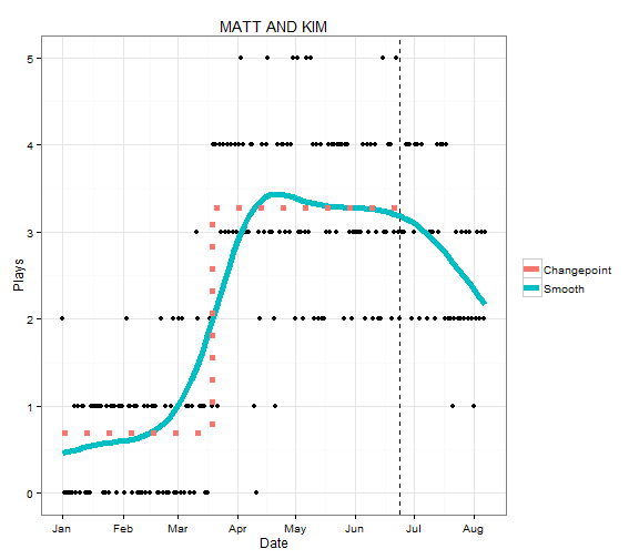
The changepoint model seems to fit the data pretty well. You can see that the average plays per day before March 19th was about 0.75, and it jumped up to 3.25 after March 19th. I think this is fairly strong evidence that CD1025 booked Matt and Kim around then and increased their exposure.

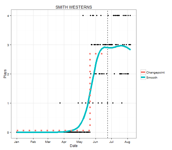
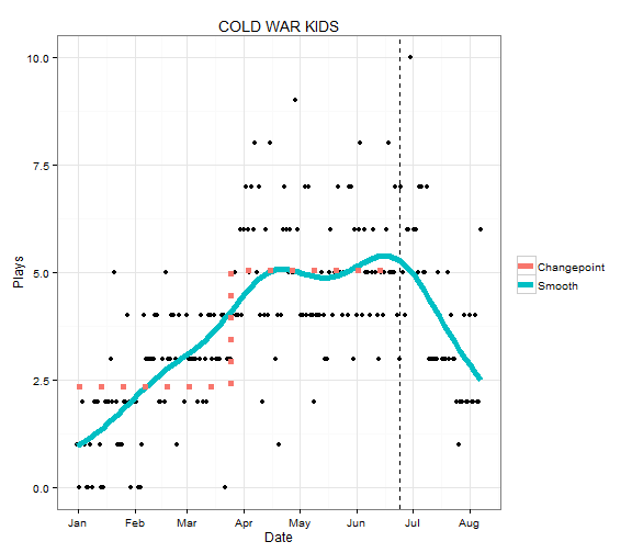
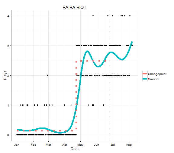
Below, I have done the same with the other headliners. Plays for Cold War Kids have increased gradually, possibly because they recently released an album. The plays for Ra Ra Riot and Smith Westerns, on the other hand, increased quite dramatically. Based on this, I think we can make pretty good guesses of when the headliners were booked, with the possible exception of Cold War Kids.

plot.plays.change(2)

plot.plays.change(3)

plot.plays.change(4)