I guess you could call this On Bayes Percentage. *cough*
Fresh off learning Bayesian techniques in one of my classes last quarter, I thought it would be fun to try to apply the method. I was able to find some examples of Hierarchical Bayes being used to analyze baseball data at Wharton.
Setting up the problem
On base percentage (OBP) is probably the most important basic offensive statistic in baseball. Getting a reliable estimate of a players true ability to get on base is therefore important. The basic problem is that the sample size we get from one season rarely has enough observations so that we are certain of a player's ability. Even though there are 162 games in a season, there is a possibility that the actual OBP is the result of luck rather than skill. Bayesian analysis will "regress" the actual observed OBP to the mean, in that if a player has a small number of plate appearances (PA) it doesn't give them very much weight and the result will be something closer to the overall (MLB) average. On the other hand, if a player has quite a few PAs then it believes that the results are not the result of luck and it gives the observations a lot of weight.
We are trying to estimate the "true" OBP of each batter. Bayesian analysis assumes that the true OBP is random. Empirical Bayes is a method of figuring out the distribution of "true" OBP using the data. OBP is times on base divided by PA. Times on base (X) for each batter is distributed binomial with n=PA and p=true OBP. We further assume that p is distributed Beta with parameters a and b. It follows from this that the marginal distribution of X is distributed according to the distribution:
gamma(a+b)*gamma(a+x)*gamma(n-x+b)*(n choose x)/(gamma(a)*gamma(b)*gamma(a+b+n))
where gamma is the gamma function.
We will estimate the parameters a and b based on the data (X), using its marginal distribution (the "empirical" part of Bayes). To do this I found that likelihood of the marginal distribution of all the batters. Then I maximized this likelihood by adjusting the parameters a and b. This is called the ML-II.
The Analysis
I used data for all non-pitchers in 2010. I assume that each player is independent. In doing that, I just have to multiply all the marginals for each player together to get the likelihood. When I do this and maximize it with respect to a and b, I get estimates that a = 83.48291 and b = 174.9038. I think this can be interpreted that prior mean (what we would assume that average OBP of a batter is before seeing him bat) is a/(a+b) = 0.323. This is pretty close to what the overall OBP of the league was (0.330). I think it makes sense that the prior is lower than the league average because batters who do well will get more opportunities and players that do poorly will get fewer. So the league average is biased high.
Below is a graph of the prior distribution and the updated posteriors of every batter. You can (sort of) see that the posteriors have tighter distributions than the prior does. (The posterior distribution of each batter in this case is the distribution of OBP after we have observed PA and the actual OBP.)

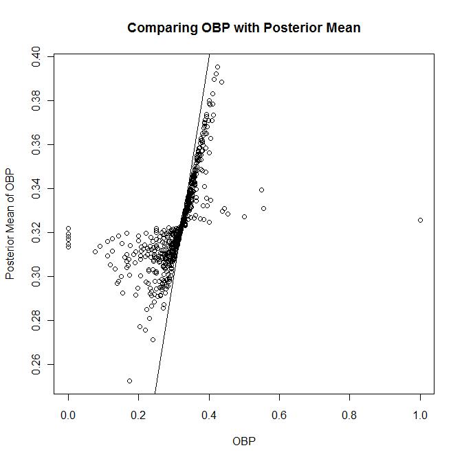
One way to see why this Bayesian analysis is useful is to compare the posterior means with the observed OBP. If someone has only a few PAs, their OBP could be very high or very low and this may mislead you into thinking that this batter is very good or bad. However, the posterior mean takes into account the number of PAs. Below is a graph comparing the two. You can see that the range of values for posterior mean is pretty small, especially compare to actual OBP.
Here is a list of the highest posterior mean OBP:
And here is a list of the lowest posterior mean OBP:
You can see that all of the posterior means are pulled closer to the overall mean (the good players look worse and the bad players look better). The order changes a little bit but not too much.
You can see the effect of sample size (PAs) by comparing Justin Morneau with Joey Votto. Morneau had a higher OBP, but Votto ended up with a higher posterior mean because he had more PAs (Votto had 648 while Morneau had 348). Here are their posterior distributions:
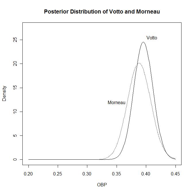
Because of the additional PAs, you can see that the distribution of Votto is a little tighter than Morneau. We are more sure that Votto is excellent than we are sure that Morneau is excellent.
Fresh off learning Bayesian techniques in one of my classes last quarter, I thought it would be fun to try to apply the method. I was able to find some examples of Hierarchical Bayes being used to analyze baseball data at Wharton.
Setting up the problem
On base percentage (OBP) is probably the most important basic offensive statistic in baseball. Getting a reliable estimate of a players true ability to get on base is therefore important. The basic problem is that the sample size we get from one season rarely has enough observations so that we are certain of a player's ability. Even though there are 162 games in a season, there is a possibility that the actual OBP is the result of luck rather than skill. Bayesian analysis will "regress" the actual observed OBP to the mean, in that if a player has a small number of plate appearances (PA) it doesn't give them very much weight and the result will be something closer to the overall (MLB) average. On the other hand, if a player has quite a few PAs then it believes that the results are not the result of luck and it gives the observations a lot of weight.
We are trying to estimate the "true" OBP of each batter. Bayesian analysis assumes that the true OBP is random. Empirical Bayes is a method of figuring out the distribution of "true" OBP using the data. OBP is times on base divided by PA. Times on base (X) for each batter is distributed binomial with n=PA and p=true OBP. We further assume that p is distributed Beta with parameters a and b. It follows from this that the marginal distribution of X is distributed according to the distribution:
gamma(a+b)*gamma(a+x)*gamma(n-x+b)*(n choose x)/(gamma(a)*gamma(b)*gamma(a+b+n))
where gamma is the gamma function.
We will estimate the parameters a and b based on the data (X), using its marginal distribution (the "empirical" part of Bayes). To do this I found that likelihood of the marginal distribution of all the batters. Then I maximized this likelihood by adjusting the parameters a and b. This is called the ML-II.
The Analysis
I used data for all non-pitchers in 2010. I assume that each player is independent. In doing that, I just have to multiply all the marginals for each player together to get the likelihood. When I do this and maximize it with respect to a and b, I get estimates that a = 83.48291 and b = 174.9038. I think this can be interpreted that prior mean (what we would assume that average OBP of a batter is before seeing him bat) is a/(a+b) = 0.323. This is pretty close to what the overall OBP of the league was (0.330). I think it makes sense that the prior is lower than the league average because batters who do well will get more opportunities and players that do poorly will get fewer. So the league average is biased high.
Below is a graph of the prior distribution and the updated posteriors of every batter. You can (sort of) see that the posteriors have tighter distributions than the prior does. (The posterior distribution of each batter in this case is the distribution of OBP after we have observed PA and the actual OBP.)
One way to see why this Bayesian analysis is useful is to compare the posterior means with the observed OBP. If someone has only a few PAs, their OBP could be very high or very low and this may mislead you into thinking that this batter is very good or bad. However, the posterior mean takes into account the number of PAs. Below is a graph comparing the two. You can see that the range of values for posterior mean is pretty small, especially compare to actual OBP.
Here is a list of the highest posterior mean OBP:
| Batter | Posterior Mean | Actual OBP |
| Joey Votto | 0.396 | 0.424 |
| Miguel Cabrera | 0.392 | 0.420 |
| Albert Pujols | 0.390 | 0.414 |
| Justin Morneau | 0.388 | 0.437 |
| Josh Hamilton | 0.383 | 0.411 |
| Prince Fielder | 0.380 | 0.401 |
| Shin-Soo Choo | 0.379 | 0.401 |
| Kevin Youkilis | 0.379 | 0.412 |
| Joe Mauer | 0.378 | 0.402 |
| Adrian Gonzalez | 0.374 | 0.393 |
| Daric Barton | 0.374 | 0.393 |
| Jim Thome | 0.373 | 0.412 |
| Paul Konerko | 0.373 | 0.393 |
| Jason Heyward | 0.373 | 0.393 |
| Matt Holliday | 0.371 | 0.390 |
| Carlos Ruiz | 0.371 | 0.400 |
| Manny Ramirez | 0.371 | 0.409 |
| Billy Butler | 0.370 | 0.388 |
| Jayson Werth | 0.370 | 0.388 |
| Ryan Zimmerman | 0.369 | 0.388 |
And here is a list of the lowest posterior mean OBP:
| Batter | Posterior Mean | Actual OBP |
| Brandon Wood | 0.252 | 0.175 |
| Pedro Feliz | 0.271 | 0.240 |
| Jeff Mathis | 0.276 | 0.219 |
| Garret Anderson | 0.277 | 0.204 |
| Adam Moore | 0.281 | 0.230 |
| Josh Bell | 0.285 | 0.224 |
| Jose Lopez | 0.286 | 0.270 |
| Peter Bourjos | 0.287 | 0.237 |
| Aaron Hill | 0.287 | 0.271 |
| Tony Abreu | 0.288 | 0.244 |
| Koyie Hill | 0.291 | 0.254 |
| Gerald Laird | 0.291 | 0.263 |
| Drew Butera | 0.291 | 0.237 |
| Jeff Clement | 0.291 | 0.237 |
| Matt Carson | 0.291 | 0.193 |
| Humberto Quintero | 0.292 | 0.262 |
| Wil Nieves | 0.292 | 0.244 |
| Matt Tuiasosopo | 0.292 | 0.234 |
| Luis Montanez | 0.292 | 0.155 |
| Cesar Izturis | 0.292 | 0.277 |
You can see that all of the posterior means are pulled closer to the overall mean (the good players look worse and the bad players look better). The order changes a little bit but not too much.
You can see the effect of sample size (PAs) by comparing Justin Morneau with Joey Votto. Morneau had a higher OBP, but Votto ended up with a higher posterior mean because he had more PAs (Votto had 648 while Morneau had 348). Here are their posterior distributions:
Because of the additional PAs, you can see that the distribution of Votto is a little tighter than Morneau. We are more sure that Votto is excellent than we are sure that Morneau is excellent.