Note: I started this post way back when the NCAA men's basketball tournament was going on, but didn't finish it until now.
Since the NCAA Men's Basketball Tournament has moved to 64 teams, a 16 seed as never upset a 1 seed. You might be tempted to say that the probability of such an event must be 0 then. But we know better than that.
In this post, I am interested in looking at different ways of estimating how the odds of winning a game change as the difference between seeds increases. I was able to download tournament data going back to the 1930s until 2012 from hoopstournament.net/Database.html. The tournament expanded to 64 teams in 1985, which is what I used for this post. I only used match ups in which one of the seeds was higher than the other because this was the easiest way to remove duplicates. (The database has each game listed twice, once with the winner as the first team and once with the loser as the first team. The vast majority (98.9%) of games had one team as a higher seed because an equal seed can only happen at the Final Four or later.)
Created by Pretty R at inside-R.org
Created by Pretty R at inside-R.org
We have no such conflict of interest, so we should try to make use of any information available. A simple way to do that is to look at the mean and standard deviation of the margin of victory when the 16 seed is playing the 1 seed. Below is a plot of the mean score difference with a ribbon for the +/- 2 standard deviations.
Created by Pretty R at inside-R.org
You can see that the ribbon includes zero for all seed differences except 15. If we assume that the score differences are roughly normal, we can calculate the probability that the score difference will be greater than 0. The results are largely the same as before, but we see now that there are no 100% estimates. Also, the 50% win percentage for a seed difference of 10 now looks a little more reasonable, albeit still out of line with the rest.
Created by Pretty R at inside-R.org
In the plot below, you can see that the logistic model predicts that the probability of winning increases throughout until reaching about 90% for the 16 versus 1. I also included a non-linear generalized additive model (GAM) model for comparison. The GAM believes that being a big favorite (16 vs 1 or 15 vs 2) gives an little boost in win probability. An advantage of modeling is that we can make predictions for match-ups that have never occurred (like a seed difference of 14).
Created by Pretty R at inside-R.org
Created by Pretty R at inside-R.org
From these models of margin of victory we can infer the probability of the higher seed winning (again, assuming normality).
Created by Pretty R at inside-R.org
This post highlights the many different ways someone can analyze the same data. Simply statistics talked a bit about this in a recent podcast. In this case, the differences are not huge, but there are noticeable changes. So the next time you read about an analysis that someone did, keep in mind all the decisions that they had to make and what type a sensitivity they would have on the results.
Created by Pretty R at inside-R.org
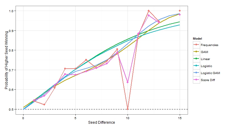
Note that the GAM functions did not have a way to easily restrict the win probability be equal to exactly 0.5 when the seed difference is 0. That is why you may notice the GAM model is a bit above 0.5 at 0.
Since the NCAA Men's Basketball Tournament has moved to 64 teams, a 16 seed as never upset a 1 seed. You might be tempted to say that the probability of such an event must be 0 then. But we know better than that.
In this post, I am interested in looking at different ways of estimating how the odds of winning a game change as the difference between seeds increases. I was able to download tournament data going back to the 1930s until 2012 from hoopstournament.net/Database.html. The tournament expanded to 64 teams in 1985, which is what I used for this post. I only used match ups in which one of the seeds was higher than the other because this was the easiest way to remove duplicates. (The database has each game listed twice, once with the winner as the first team and once with the loser as the first team. The vast majority (98.9%) of games had one team as a higher seed because an equal seed can only happen at the Final Four or later.)
library(ggplot2); theme_set(theme_bw())
brackets=read.csv("NCAAHistory.csv")

# use only data from 1985 on in which the first team has the higher seed
brackets=subset(brackets,Seed<Opponent.Seed & Year>=1985 & Round!="Opening Round")

brackets$SeedDiff=abs(brackets$Opponent.Seed-brackets$Seed)
brackets$HigherSeedWon=ifelse(brackets$Opponent.Seed>brackets$Seed,brackets$Wins,brackets$Losses)
brackets$HigherSeedScoreDiff=ifelse(brackets$Opponent.Seed>brackets$Seed,1,-1)*(brackets$Score-brackets$Opponent.Score)
Use Frequencies
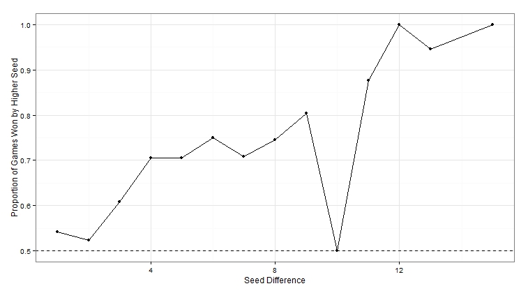
The first way is the most simple: look at the historical records when a 16 seed is playing a 1 seed (where the seed difference is 15). As you can see from the plot below, when the seed difference is 15, the higher seeded team has won every time. This is also true when the seed difference is 12, although there have only been 4 games in this scenario. Another oddity is that when the seed difference is 10, the higher seed only has only won 50% of the time. Again, this is largely due to the fact that there have only been 6 games with this seed difference.seed.diffs=sort(unique(brackets$SeedDiff))
win.pct=sapply(seed.diffs,function(x) mean(brackets$HigherSeedWon[brackets$SeedDiff==x]))
ggplot(data=data.frame(seed.diffs,win.pct),aes(seed.diffs,win.pct))+geom_point()+
geom_hline(yintercept=0.5,linetype=2)+
geom_line()+labs(x="Seed Difference",y="Proportion of Games Won by Higher Seed")
Use Score Difference
In many applications, it has been shown that using margin of victory is much more reliable than just wins and losses. For example, in the computer ranking of College Football teams, using score differences is more accurate, but outlawed for fear that teams would run up the score on weaker opponents. So the computer rankings are not as strong as they could be.We have no such conflict of interest, so we should try to make use of any information available. A simple way to do that is to look at the mean and standard deviation of the margin of victory when the 16 seed is playing the 1 seed. Below is a plot of the mean score difference with a ribbon for the +/- 2 standard deviations.
seed.diffs=sort(unique(brackets$SeedDiff))
means=sapply(seed.diffs,function(x) mean(brackets$HigherSeedScoreDiff[brackets$SeedDiff==x]))
sds=sapply(seed.diffs,function(x) sd(brackets$HigherSeedScoreDiff[brackets$SeedDiff==x]))
ggplot(data=data.frame(seed.diffs,means,sds),aes(seed.diffs,means))+
  geom_ribbon(aes(ymin=means-2*sds,ymax=means+2*sds),alpha=.5)+geom_point()+geom_line()+
  geom_hline(yintercept=0,linetype=2)+
  labs(x="Seed Difference",y="Margin of Victory by Higher Seed")
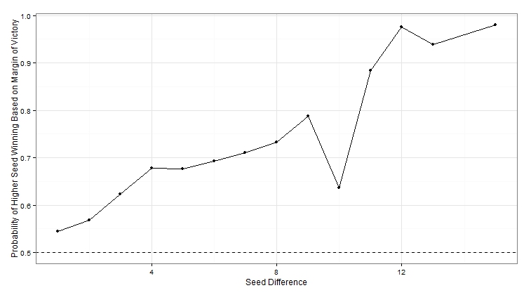
You can see that the ribbon includes zero for all seed differences except 15. If we assume that the score differences are roughly normal, we can calculate the probability that the score difference will be greater than 0. The results are largely the same as before, but we see now that there are no 100% estimates. Also, the 50% win percentage for a seed difference of 10 now looks a little more reasonable, albeit still out of line with the rest.
ggplot(data=data.frame(seed.diffs,means,sds),aes(seed.diffs,1-pnorm(0,means,sds)))+
  geom_point()+geom_line()+geom_hline(yintercept=0.5,linetype=2)+
  labs(x="Seed Difference",y="Probability of Higher Seed Winning Based on Margin of Victory")
Model Win Percentage as a Function of Seed Difference
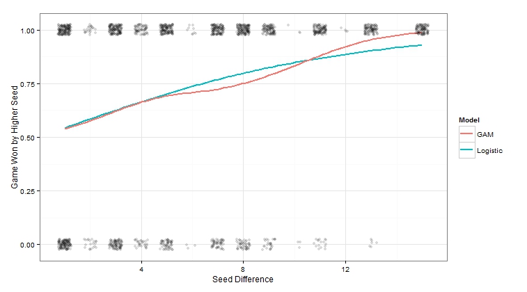
It is always good to incorporate as much knowledge as possible into an analysis. In this case, we have information on other games besides the 16 versus 1 seed game which help us estimate the 16 versus 1 game. For example, it is reasonable to assume that the larger the difference in seed is, the more likely the higher seed will win. We can build a logistic regression model which looks at all of the outcomes of all of the games and predicts the probability of winning based on the difference in seed. When the two teams have the same seed, I enforced the probability of the higher seed winning to be 0.5 by making the intercept 0.In the plot below, you can see that the logistic model predicts that the probability of winning increases throughout until reaching about 90% for the 16 versus 1. I also included a non-linear generalized additive model (GAM) model for comparison. The GAM believes that being a big favorite (16 vs 1 or 15 vs 2) gives an little boost in win probability. An advantage of modeling is that we can make predictions for match-ups that have never occurred (like a seed difference of 14).
ggplot(data=brackets,aes(SeedDiff,HigherSeedWon))+
  stat_smooth(method="gam",family="binomial",se=F,formula=y~0+x,aes(colour="Logistic"),size=1)+
  stat_smooth(method="gam",family="binomial",se=F,formula=y~s(x),aes(colour="GAM"),size=1)+
  geom_jitter(alpha=.15,position = position_jitter(height = .025,width=.25))+
  labs(x="Seed Difference",y="Game Won by Higher Seed",colour="Model")
Model Score Difference as a Function of Seed Difference
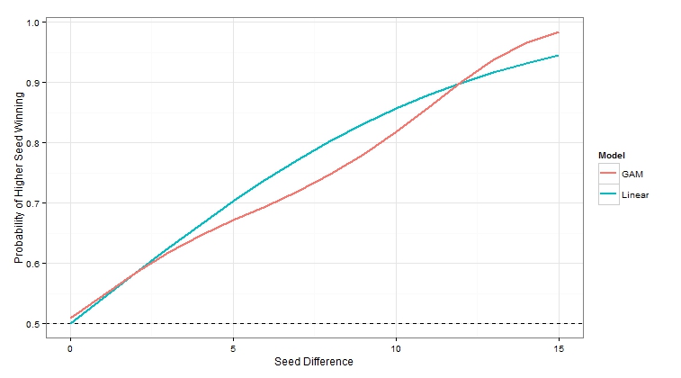
We can also do the same thing with margin of victory. Here, I constrain the linear model to have an intercept of 0, meaning that two teams with the same seed should be evenly matched. Again, I included the GAM fit for comparison. The interpretations are similar to before, in that it seems that there is an increase in margin of victory for the heavily favored teams.ggplot(data=brackets,aes(SeedDiff,HigherSeedScoreDiff))+
stat_smooth(method="lm",se=F,formula=y~0+x,aes(colour="Linear"),size=1)+
stat_smooth(method="gam",se=F,formula=y~s(x),aes(colour="GAM"),size=1)+
geom_jitter(alpha=.25,position = position_jitter(height = 0,width=.25))+
labs(x="Seed Difference",y="Margin of Victory by Higher Seed",colour="Model")
From these models of margin of victory we can infer the probability of the higher seed winning (again, assuming normality).
library(gam)
lm.seed=lm(HigherSeedScoreDiff~0+SeedDiff,data=brackets)
gam.seed=gam(HigherSeedScoreDiff~s(SeedDiff),data=brackets)

pred.lm.seed=predict(lm.seed,data.frame(SeedDiff=0:15),se.fit=TRUE)
pred.gam.seed=predict(gam.seed,data.frame(SeedDiff=0:15),se.fit=TRUE)
se.lm=sqrt(mean(lm.seed$residuals^2))
se.gam=sqrt(mean(gam.seed$residuals^2))

df1=data.frame(SeedDiff=0:15,ProbLM=1-pnorm(0,pred.lm.seed$fit,sqrt(se.lm^2+pred.lm.seed$se.fit^2)),
               ProbGAM=1-pnorm(0,pred.gam.seed$fit,sqrt(se.gam^2+pred.gam.seed$se.fit^2)))
ggplot(df1)+geom_hline(yintercept=0.5,linetype=2)+
  geom_line(aes(SeedDiff,ProbLM,colour="Linear"),size=1)+
  geom_line(aes(SeedDiff,ProbGAM,colour="GAM"),size=1)+
  labs(x="Seed Difference",y="Probability of Higher Seed Winning",colour="Model")
Summary
Putting all of the estimates together, you can easily spot the differences between the models. The two assumptions that just used the data between specific seeds look pretty similar. It looks like using score differential is a little more reasonable of the two. The two GAMs have a similar trend and so did the linear and logistic models. If someone asks you what the probability that a 16 seed beats a 1 seed, you have at least 6 different answers.This post highlights the many different ways someone can analyze the same data. Simply statistics talked a bit about this in a recent podcast. In this case, the differences are not huge, but there are noticeable changes. So the next time you read about an analysis that someone did, keep in mind all the decisions that they had to make and what type a sensitivity they would have on the results.
logit.seed=glm(HigherSeedWon~0+SeedDiff,data=brackets,family=binomial(logit))
logit.seed.gam=gam(HigherSeedWon~s(SeedDiff),data=brackets,family=binomial(logit))

df2=data.frame(SeedDiff=0:15,
               ProbLM=1-pnorm(0,pred.lm.seed$fit,sqrt(se.lm^2+pred.lm.seed$se.fit^2)),
               ProbGAM=1-pnorm(0,pred.gam.seed$fit,sqrt(se.gam^2+pred.gam.seed$se.fit^2)),
               ProbLogit=predict(logit.seed,data.frame(SeedDiff=0:15),type="response"),
               ProbLogitGAM=predict(logit.seed.gam,data.frame(SeedDiff=0:15),type="response"))
df2=merge(df2,data.frame(SeedDiff=seed.diffs,ProbFreq=win.pct),all.x=T)
df2=merge(df2,data.frame(SeedDiff=seed.diffs,ProbScore=1-pnorm(0,means,sds)),all.x=T)
ggplot(df2,aes(SeedDiff))+geom_hline(yintercept=0.5,linetype=2)+
  geom_line(aes(y=ProbLM,colour="Linear"),size=1)+
  geom_line(aes(y=ProbGAM,colour="GAM"),size=1)+
  geom_line(aes(y=ProbLogit,colour="Logistic"),size=1)+
  geom_line(aes(y=ProbLogitGAM,colour="Logistic GAM"),size=1)+
  geom_line(aes(y=ProbFreq,colour="Frequencies"),size=1)+
  geom_line(aes(y=ProbScore,colour="Score Diff"),size=1)+
  geom_point(aes(y=ProbFreq,colour="Frequencies"),size=3)+
  geom_point(aes(y=ProbScore,colour="Score Diff"),size=3)+
  labs(x="Seed Difference",y="Probability of Higher Seed Winning",colour="Model")

ggplot(df2)+geom_hline(yintercept=0.5,linetype=2)+
  geom_point(aes(x=SeedDiff,y=ProbFreq,colour="Frequencies"),size=1)
Note that the GAM functions did not have a way to easily restrict the win probability be equal to exactly 0.5 when the seed difference is 0. That is why you may notice the GAM model is a bit above 0.5 at 0.
