That title is quite a mouthful. This quarter, I have been reading papers on Spectral Clustering for a reading group. The basic goal of clustering is to find groups of data points that are similar to each other. Also, data points in one group should be dissimilar to data in other clusters. This way you can summarize your data by saying there are a few groups to consider instead of all the points. Clustering is an unsupervised learning method in that there are no "true" groups that you are comparing the clusters to.
There are many ways to do this, two of the most popular are k-means and hierarchical clustering. Spectral clustering is nice because it gives you as much flexibility as you want to define how pairs of data points are similar or dissimilar. K-means only works well for data that are grouped in elliptically shaped, whereas spectral clustering can theoretically work well for any group. For example, the data in this image is easily clustered by spectral, but would not be by k-means. The flexibility of spectral clustering can also be a burden in that there are an infinite ways to group points.
The basic idea (and all the flexibility) behind spectral clustering is that you define the similarity between any two data points however you want, and put them in a matrix. So if you have 100 data points, you will end up with a 100x100 matrix, where the rth row and cth column is the similarity between the rth data point and the cth data point. You can define "similarity" any way you want. Popular methods are Euclidean distance, a kernel function of the Euclidean distance, or a k nearest neighbors approach.
Once you have the similarity matrix, you need to create a normalized/unnormalized Laplacian matrix, then calculate the eigenvectors and eigenvalues of the the Laplacian. Finally, use the k-means algorithm on the eigenvalues corresponding to the k smallest eigenvectors. This will give you k clusters (something else you need to specify).
The other day, someone in my office was working a project of Image Segmentation (a topic I know nothing about) for a machine learning class. I thought this would be a perfect application for spectral clustering because you can define similarity of pixels in terms of both the contrast of the pixel as well as the proximity to nearby pixels. I downloaded a few pictures from the Berkeley Segmentation Dataset Benchmark website.
One thing I quickly found was that even these moderately sized pictures were too big to create a similarity matrix for in R. A typical image is 481x321=154401 pixels. So a similarity matrix between all the pixels would be 154401x154401=23 billion elements. R only allows 2^31-1=2.1 billion elements in a matrix. Even if I could create the matrix, it would take forever to calculate the eigenvectors and eigenvalues. [Note: Some people from my department actually tackled this exact problem using sampling methods.]
So I had to reduce the size of the image. For this I just created an image of a factor of the original dimension (about 10 to 20 times smaller), and averaged the contrast of all the points that were collapsed. I also experimented with smoothing the image first and then doing the averaging In some cases it helped in some it hurt, I think.
For example here is an original picture.
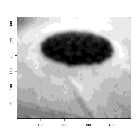
Then I smoothed using the image.smooth function of the fields package.
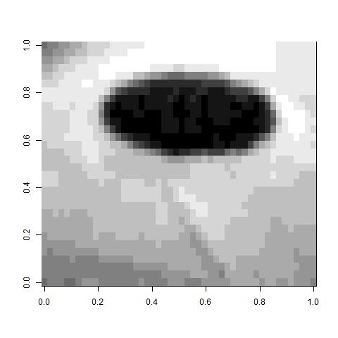
Then I reduced the dimension by a factor of 10 and averaged the original pixels. The resulting image is below. You can see there is a decent loss of information in the averaging.
Finally, for the similarity, I only considered pixels that were within 3 horizontally or vertically to be similar (otherwise 0). Also, for those within 3, I used a Gaussian kernel of the difference in contrast with variance equal to 0.01. I chose this number because the variance in the data was about 0.01. Varying both of these parameters wildly affected quality of the results. I also tried using a k nearest neighbors similarity and I did not get any good results. Hence, you can see both the positive and negative of the flexibility.
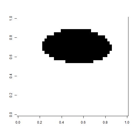
Anyway, here are the two clusters (white and black) using the unnormalized Laplacian.
It looks very good and encouraging for future problems. As stated before, however, I am not sure how to determine the parameters for a generic problem.
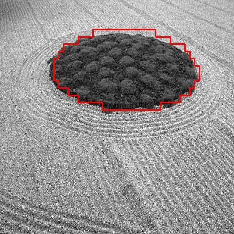
Overlaying the cluster on the original image, you can see the two segments of the image clearly. You can also see the loss in fidelity due to reducing the size of the image.
Here are a couple of other examples that worked well. With the airplane one, in particular, you can see that the clustering was able to identify an unusual shape. I was not able to get it to work well with more than two clusters, although I only tried one image that was not that easy.
For posterity, here is the code I used.
############
# Import the image
############
library(jpeg)
# http://www.eecs.berkeley.edu/Research/Projects/CS/vision/bsds/BSDS300/html/images/plain/normal/gray/86016.jpg
rawimg=readJPEG("segment.jpeg")
rawimg=t(rawimg)
rawimg=rawimg[,ncol(rawimg):1]
image(rawimg,col = grey((0:12)/12))
############
# Smooth the image
############
library(fields)
smoothimg=image.smooth(rawimg,theta=2)
image(smoothimg,col = grey((0:12)/12))
############
# Reduce Size of Image
############
olddim=dim(rawimg)
newdim=c(round(olddim/10))
prod(newdim)>2^31
img=matrix(NA,newdim[1],newdim[2])
for (r in 1:newdim[1]) {
centerx=(r-1)/newdim[1]*olddim[1]+1
lowerx=max(1,round(centerx-olddim[1]/newdim[1]/2,0))
upperx=min(olddim[1],round(centerx+olddim[1]/newdim[1]/2,0))
for (c in 1:newdim[2]) {
centery=(c-1)/newdim[2]*olddim[2]+1
lowery=max(1,round(centery-olddim[2]/newdim[2]/2,0))
uppery=min(olddim[2],round(centery+olddim[2]/newdim[2]/2,0))
img[r,c]=mean(smoothimg$z[lowerx:upperx,lowery:uppery])
}
}
image(img,col = grey((0:12)/12))
############
# Convert matrix to vector
############
imgvec=matrix(NA,prod(dim(img)),3)
counter=1
for (r in 1:nrow(img)) {
for (c in 1:ncol(img)) {
imgvec[counter,1]=r
imgvec[counter,2]=c
imgvec[counter,3]=img[r,c]
counter=counter+1
}
}
############
# Similarity Matrix
############
pixdiff=2
sigma2=.01 #var(imgvec[,3])
simmatrix=matrix(0,nrow(imgvec),nrow(imgvec))
for(r in 1:nrow(imgvec)) {
cat(r,"out of",nrow(imgvec),"\n")
simmatrix[r,]=ifelse(abs(imgvec[r,1]-imgvec[,1])<=pixdiff & abs(imgvec[r,2]-imgvec[,2])<=pixdiff,exp(-(imgvec[r,3]-imgvec[,3])^2/sigma2),0)
}
############
# Weighted and Unweighted Laplacian
############
D=diag(rowSums(simmatrix))
Dinv=diag(1/rowSums(simmatrix))
L=diag(rep(1,nrow(simmatrix)))-Dinv %*% simmatrix
U=D-simmatrix
############
# Eigen and k-means
############
evL=eigen(L,symmetric=TRUE)
evU=eigen(U,symmetric=TRUE)
kmL=kmeans(evL$vectors[,(ncol(simmatrix)-1):(ncol(simmatrix)-0)],centers=2,nstart=5)
segmatL=matrix(kmL$cluster-1,newdim[1],newdim[2],byrow=T)
if(max(segmatL) & sum(segmatL==1)<sum(segmatL==0)) {segmatL=abs(segmatL-1)}
kmU=kmeans(evU$vectors[,(ncol(simmatrix)-1):(ncol(simmatrix)-0)],centers=2,nstart=5)
segmatU=matrix(kmU$cluster-1,newdim[1],newdim[2],byrow=T)
if(max(segmatU) &sum(segmatU==1)<sum(segmatU==0)) {segmatU=abs(segmatU-1)}
############
# Plotting the clusters
############
image(segmatL, col=grey((0:15)/15))
image(segmatU, col=grey((0:12)/12))
############
# Overlaying the original and the clusters
############
image(seq(0,1,length.out=olddim[1]),seq(0,1,length.out=olddim[2]),rawimg,col = grey((0:12)/12),xlim=c(-.1,1.1),ylim=c(-.1,1.1),xlab="",ylab="")
segmat=segmatU
linecol=2
linew=3
for(r in 2:newdim[1]) {
for (c in 2:newdim[2]) {
if(abs(segmat[r-1,c]-segmat[r,c])>0) {
xloc=(r-1)/(newdim[1])
ymin=(c-1)/(newdim[2])
ymax=(c-0)/(newdim[2])
segments(xloc,ymin,xloc,ymax,col=linecol,lwd=linew)
}
if(abs(segmat[r,c-1]-segmat[r,c])>0) {
yloc=(c-1)/(newdim[2])
xmin=(r-1)/(newdim[1])
xmax=(r-0)/(newdim[1])
segments(xmin,yloc,xmax,yloc,col=linecol,lwd=linew)
}
}
}


