In a previous post, I showed you how to scrape playlist data from Columbus, OH alternative rock station CD102.5. Since it's the end of the year and best-of lists are all the fad, I thought I would share the most popular songs and artists of the year, according to this data. In addition to this, I am going to make an interactive graph using Shiny, where the user can select an artist and it will graph the most popular songs from that artist.
First off, I am assuming that you have scraped the appropriate data using the code from the previous post.
Next, I will select just the data from 2013 and find the songs that were played most often.
The top 10 songs are the following:
I will make a plot similar to the plots made in the last post to show when the top 5 songs were played throughout the year.
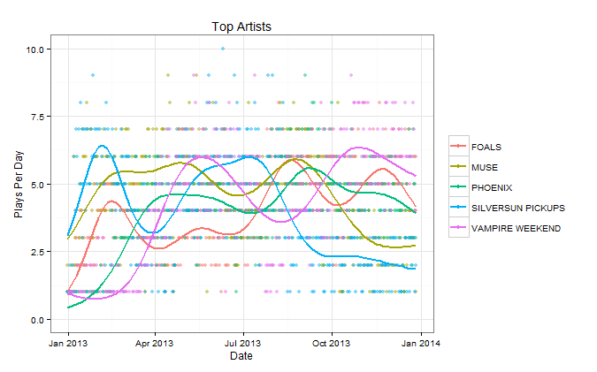
I can similarly summarize by artist as well.
Finally, I wrote a Shiny interactive app. They are surprisingly easy to create and if you are thinking about experimenting with it, I suggest you try it. I will leave the code for the app in a gist. In the app, you can enter any artist you want, and it will show you the most popular songs on CD102.5 for that artist. You can also select the number of songs that it plots with the slider.
For example, even though Muse did not have one of the most popular songs of the year, they were still the band that was played the most. By typing in "MUSE" in the Artist text input, you will get the following output.
They had two songs that were very popular this year and a few others that were decently popular as well.
Play around with it and let me know what you think.
First off, I am assuming that you have scraped the appropriate data using the code from the previous post.
library(lubridate)
library(sqldf)

playlist=read.csv("CD101Playlist.csv",stringsAsFactors=FALSE)
dates=mdy(substring(playlist[,3],nchar(playlist[,3])-9,nchar(playlist[,3])))
times=hm(substring(playlist[,3],1,nchar(playlist[,3])-10))
playlist$Month=ymd(paste(year(dates),month(dates),"1",sep="-"))
playlist$Day=dates
playlist$Time=times
playlist=playlist[order(playlist$Day,playlist$Time),]
Next, I will select just the data from 2013 and find the songs that were played most often.
playlist=subset(playlist,Day>=mdy("1/1/13"))
playlist$ArtistSong=paste(playlist$Artist,playlist$Song,sep="-")
top.songs=sqldf("Select ArtistSong, Count(ArtistSong) as Num
      From playlist
      Group By ArtistSong
      Order by Num DESC
      Limit 10")
The top 10 songs are the following:
                              Artist-Song Number Plays
1  FITZ AND THE TANTRUMS-OUT OF MY LEAGUE 809
2                      ALT J-BREEZEBLOCKS 764
3              COLD WAR KIDS-MIRACLE MILE 759
4                      ATLAS GENIUS-IF SO 750
5                         FOALS-MY NUMBER 687
6                         MS MR-HURRICANE 679
7       THE NEIGHBOURHOOD-SWEATER WEATHER 657
8           CAPITAL CITIES-SAFE AND SOUND 646
9             VAMPIRE WEEKEND-DIANE YOUNG 639
10             THE FEATURES-THIS DISORDER 632
I will make a plot similar to the plots made in the last post to show when the top 5 songs were played throughout the year.
plays.per.day=sqldf("Select Day, Count(Artist) as Num
      From playlist
      Group By Day
      Order by Day")

playlist.top.songs=subset(playlist,ArtistSong %in% top.songs$ArtistSong[1:5])

song.per.day=sqldf(paste0("Select Day, ArtistSong, Count(ArtistSong) as Num
                          From [playlist.top.songs]
                          Group By Day, ArtistSong
                          Order by Day, ArtistSong"))
dspd=dcast(song.per.day,Day~ArtistSong,sum,value.var="Num")

song.per.day=merge(plays.per.day[,1,drop=FALSE],dspd,all.x=TRUE)
song.per.day[is.na(song.per.day)]=0

song.per.day=melt(song.per.day,1,variable.name="ArtistSong",value.name="Num")
song.per.day$Alpha=ifelse(song.per.day$Num>0,1,0)

library(ggplot2)
ggplot(song.per.day,aes(Day,Num,colour=ArtistSong))+geom_point(aes(alpha=Alpha))+
  geom_smooth(method="gam",family=poisson,formula=y~s(x),se=F,size=1)+
  labs(x="Date",y="Plays Per Day",title="Top Songs",colour=NULL)+
  scale_alpha_continuous(guide=FALSE,range=c(0,.5))+theme_bw()
I can similarly summarize by artist as well.
top.artists=sqldf("Select Artist, Count(Artist) as Num
                From playlist
                Group By Artist
                Order by Num DESC
                Limit 10")
                    Artist  Num
1                     MUSE 1683
2          VAMPIRE WEEKEND 1504
3        SILVERSUN PICKUPS 1442
4                    FOALS 1439
5                  PHOENIX 1434
6            COLD WAR KIDS 1425
7                JAKE BUGG 1316
8  QUEENS OF THE STONE AGE 1296
9                    ALT J 1233
10     OF MONSTERS AND MEN 1150
playlist.top.artists=subset(playlist,Artist %in% top.artists$Artist[1:5])

artists.per.day=sqldf(paste0("Select Day, Artist, Count(Artist) as Num
                          From [playlist.top.artists]
                          Group By Day, Artist
                          Order by Day, Artist"))
dspd=dcast(artists.per.day,Day~Artist,sum,value.var="Num")

artists.per.day=merge(plays.per.day[,1,drop=FALSE],dspd,all.x=TRUE)
artists.per.day[is.na(artists.per.day)]=0

artists.per.day=melt(artists.per.day,1,variable.name="Artist",value.name="Num")
artists.per.day$Alpha=ifelse(artists.per.day$Num>0,1,0)

ggplot(artists.per.day,aes(Day,Num,colour=Artist))+geom_point(aes(alpha=Alpha))+
  geom_smooth(method="gam",family=poisson,formula=y~s(x),se=F,size=1)+
  labs(x="Date",y="Plays Per Day",title="Top Artists",colour=NULL)+
  scale_alpha_continuous(guide=FALSE,range=c(0,.5))+theme_bw()
Finally, I wrote a Shiny interactive app. They are surprisingly easy to create and if you are thinking about experimenting with it, I suggest you try it. I will leave the code for the app in a gist. In the app, you can enter any artist you want, and it will show you the most popular songs on CD102.5 for that artist. You can also select the number of songs that it plots with the slider.
For example, even though Muse did not have one of the most popular songs of the year, they were still the band that was played the most. By typing in "MUSE" in the Artist text input, you will get the following output.
They had two songs that were very popular this year and a few others that were decently popular as well.
Play around with it and let me know what you think.


